Influence Functions in XAI

Table of Contents

1. Introduction
2. Influence Functions
   • 2.1 Efficiently Calculating Influence Functions
     • 2.1.1 Problems with LiSSA Algorithm
   • 2.2 Experiments & Results
3. Faster Influence Functions with FastIF
4. Fragility of Influence Functions
   • 4.1 Experiments
     • 4.1.1 Understanding IF when the exact Hessian can be computed
       • 4.1.1.1 Effect of the Weight Decay
       • 4.1.1.2 Effect of the Depth
       • 4.1.1.3 Effect of the Width
       • 4.1.1.4 Effect of the Inverse-Hessian Vector Product
     • 4.1.2 Understanding IF for Shallow CNN
     • 4.1.3 Understanding IF for Deep Architectures
     • 4.2 Conclusion

1. Introduction

In the ever-evolving field of deep learning, the need for understanding the model decision becomes more important each day. To fully incorprate deep learning systems into a critical decision systems such as self-driving cars and medical AI supervisors, tracing back the algorithm into its’ data point gives us a lot of understanding about the decision system itself. However deep learning systems are often blackboxes.

One simple question arises from these concerns:

One can find how influential a data point $x$is on the decision of the model $f_\theta(x^*)$ where $x^*$is a point not seen in the dataset by asking:

A simple way to calculate this effect is to retrain your model without the data point $x$: however this is a very costly approach as current deep learning models usually takes a long time to train.

Influence Functions approximates the effect of how influential a point is with other points. In this blog post, we will formally defining the influential functions, their mathematical formulations, their advantages and their problems.

2. Influence Functions

Koh et al. utilize influence functions, a statistical tool, to sidestep the computationally intensive process of retraining models. They focus on estimating the impact of a single data point on a model’s decision-making. Firstly, they assume the model parameters $θ$ are twice-differentiable and strictly convex. This is an important fact to get a good estimate of influence and we will revisit this topic on the later sections. Given a model that maps inputs from a space $\mathcal X$ to outputs in $\mathcal Y$ , using training points $(z_i,...,z_n)$ where $z_i = (x_i,y_i)\in \mathcal X \times \mathcal Y$, they define a loss function $L$ parameterized by $θ$:

The influence of a data point $x$ is quantified by the change in model parameters upon removing the point:

To avoid retraining for $\hat \theta^{−z}$​, they propose approximating this by assessing a point $z$‘s sensitivity to changes in the loss function. Formally, for a given $\epsilon$, they define:

Notice that setting $\epsilon = -\frac{1}{n}$ approximates the effect of excluding the $z$ from the training set. Define the effect of upweighting the point $z$ by the $\epsilon$ as:

To show the closed form expression of this function, authors start by defining empirical risk as $R(\theta) = \frac{1}{n}\sum_{i=1}^n L(z_i, \theta)$. We can rewrite the equation $(2.3)$ by plugging in our risk function:

The quantity we seek $\frac{\partial \hat \theta_{\epsilon,z}}{\partial \epsilon}$ can be computed as:

where $\Delta_\epsilon = \hat \theta_{\epsilon,z} - \hat \theta$ as $\frac{\partial \hat \theta}{\partial \epsilon}=0$. Since $\hat \theta_{\epsilon,z}$ is the minimizer of the $(2.4)$, first-order optimality condition holds:

Since $\lim_{\epsilon \rightarrow 0} L(z, \hat \theta_{\epsilon,z}) = L(z, \hat \theta)$, we have $\lim_{\epsilon \rightarrow 0} \hat \theta_{\epsilon,z} = \hat \theta$. Performing the Taylor approximation to the right-hand side of the equation $(2.5)$, we get:

where the $o(||\nabla_\epsilon||)$ error term is dropped. Get the $\Delta_\epsilon$ approximation by readjusting the equation $(2.6)$:

Since $\epsilon \rightarrow 0$ and $\nabla R(\hat \theta) = 0$ as $\hat \theta$ minimizes the risk function $R(\theta)$, we can write the equation $(2.7)$ as

Rewriting the $\nabla^2 R(\hat \theta) = H_{\hat \theta}$ where

we compute the $\mathcal I_{up,params}(z)$ as

Now the effect of upweighting the point $z$ is derived, let us calculate the effect of upweighting the point $z$ on the loss function of the test point $z_{test}$ by using the chain rule:

Basically, $\mathcal I_{up,loss}(z,z_{test})$ approximates the influence of the point $z$ on the loss of point $z_{test}$ and is called influence function ¹. To see why this statement holds, lets closely inspect the expression:

Having derived a closed-form solution for influence functions, which approximate the true impact of a data point $z$ on the loss for $z_{test}$, we face a significant computational challenge. The Hessian calculation, necessitating all data points, escalates in complexity to $\mathcal{O}(np^2)$, with $p$ denoting the total parameter count. This complexity is further amplified by the need to invert such a sizable matrix. Our next discussion will explore strategies for efficiently approximating the inverse of the Hessian matrix, aiming to mitigate this computational burden.

2.1 Efficiently calculating the influence

Inverting the Hessian of the empirical risk takes $O(np^2 + p^3)$operations where $n$ is the number of points and $p$is the dimension of the weights $\theta \in \mathbb R^p$. To efficiently compute the inverse of a Hessian, authors use Hessian-vector products (HVPs) to efficiently approximate:

If $s_{test}$is precomputed, calculating influence of a point $z$ on $z_{test}$ would be fast as we would only need to compute $\nabla L(z,\hat \theta)$:

Authors discuss two algorithms in order to efficiently compute $s_{test}$. First idea is to use conjugate gradients method, in which the assumption of Hessian being a convex is used to transform the problem into a optimization problem. However this method can still be slow.

The second algorithm, LiSSA (Linear (time) Stochastic Second-Order Algorithm) ² uses the well known fact about the inverse of a positive-definite matrix with $||A|| < 1$ (since this is equal to the largest absolute eigenvalue, it means all eigenvalues value should be smaller than $1$) to calculate the inverse of the matrix as:

This is basically recursive reformulation of the Taylor expansion. The first $j$ terms can of the expension can be expressed as:

where $\lim_{j \rightarrow \infty} H_j^{-1} = H^{-1}$ if the assumptions are satisfied. Using the fact that $(I - H)^0 = I$, we can adjust our equation to get

Notice how we can compute this iteratively; by simply storing the previous estimation of the Hessian. After sampling $t$ points $z_{s_1},...,z_{s_t}$ from a uniform distribution, authors suggest that $H$ can be approximated stochastically with a single point $\tilde H = \nabla_\theta^2 L(z_i, \hat \theta)$.

where $\tilde H_0^{-1}v = v$ is set. With a large $t$, $\tilde H_t$ stabilizes. Authors also suggest to use this procedure $r$ times and take the average of the results. This algorithm can be used to compute $\mathcal I_{up,loss}(z_i,z_{test})$ in $O(np + rtp)$ time. To understand more about this sections, it is suggested to study the original LiSSA algorithm for estimating Hessian inverse ².

2.1.1 Problems with LiSSA algorithm

One problem with this approach is that it assumes that the norm $||A|| < 1$ holds. Also another problem occurs if the matrix $H$ is not invertible, however it is already claimed at Section 2 that loss function is strictly convex, which makes the $H$ positive definite and invertible. We left with the problem of having an eigenvalue with maximum absolute value larger than $1$. For this problem, one can use damping & scaling method to make the matrix satisfies the convergence criteria. This approach tries to find $d$ and $s$ such that:

is both positive definite and has bounded eigenvalues that are smaller than $1$. For very small $d$ we can approximate $(dI + H/s)^{-1}$ using LiSSA algorithm and approximate the inverse of Hessian as:

2.2. Experiments & Results

WIP

3. Faster Influence Functions

WIP

4. Fragility of Influence Functions

We have covered some basic aspects of the influence functions. In practice, however, the positive definiteness and convexity assumption fails due to non-convex loss functions and complex structures. Also in most of the cases, exact Hessian is not computed we require an approximation. This bring us to the next topic of discussing whether influence functions are fairly accurate for more deeper, complex networks.

Basu et al. ³ works on the fragility of influence functions shows that hyperparameters and network structure greatly affects the quality of approximating the re-training of a model without a particular input via influence functions.

Taylor approximation around the optimal parameters, as shown in the equation (2.7), can be inaccurate if the parameter space is varies a lot within its neighbourhood. Particularly, this happens for non-convex loss functions. Authors investigate the effects of the weight decay regularization, network depth and height.

4.1 Experiments

The study investigates the effectiveness of influence functions across datasets of varying complexity, starting with the Iris dataset and advancing through MNIST, CIFAR-10, to ImageNet, to assess their accuracy in deep learning models. It evaluates these influence estimates using both Pearson and Spearman correlation methods, focusing on the latter for its relevance in ranking influential examples by importance. This approach allows for a detailed analysis of how well influence functions can identify and rank influential training points in relation to a specific test point, providing insights into their scalability and utility in interpreting deep learning models.

4.1.1 Understanding IF when the exact Hessian can be computed

The computation of the Hessian matrix and its inverse is a computationally intensive task, particularly in the context of large neural networks. Due to this complexity, iterative algorithms are often employed to approximate the Hessian and its inverse, providing a balance between computational feasibility and the accuracy of influence function (IF) estimates. In the initial experiments conducted on the Iris dataset, which features a small feed-forward neural network, the authors took advantage of the dataset’s manageability to compute the exact Hessian. This approach is advantageous as it allows for a precise comparison between the influence functions’ estimates and the true influence exerted by training points on the model’s predictions. The exact computation of the Hessian in this context serves as a valuable baseline, offering clear insights into the accuracy and reliability of influence functions in simpler neural network settings before extending the analysis to more complex models and larger datasets where approximations are necessary.

4.1.1.1 Effect of the Weight Decay

Weight decay is a common regularization technique that pushes the model towards a simpler hypothesis space. With their extensive experiments, authors show that weight decay has a large effect on the high quality influence estimates. To be more precise, they found that for the small feed-forward neural networks that is trained with weight-decay greatly increases the Spearman correlation between the influence estimates and the ground-truth estimates.

4.1.1.2 Effect of the Depth

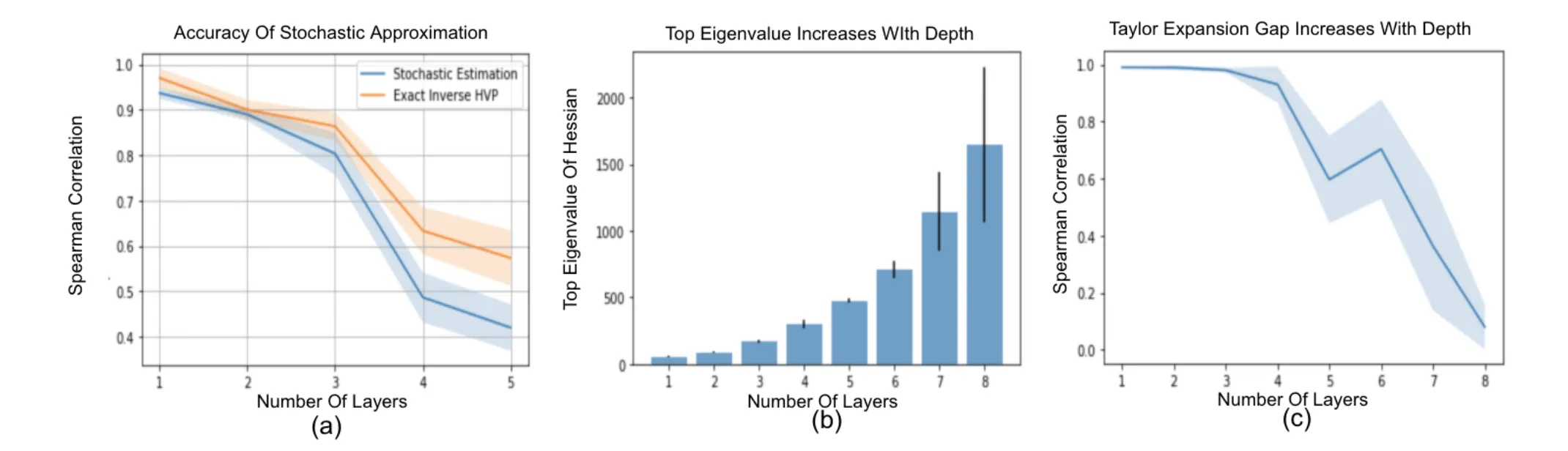
The study highlights the significant impact of network depth on the accuracy of influence estimates, observing that deeper networks (beyond 8 layers) exhibit a notable decline in Spearman correlation with ground-truth parameter changes. This decline suggests that as network depth increases, the ability of influence functions to accurately approximate parameter changes diminishes. The research quantifies this by comparing the norm of true parameter changes (obtained through re-training) against approximate changes predicted by influence functions, especially focusing on the most influential examples. A consistent trend emerges where the approximation error widens with network depth, particularly exceeding 5 layers, alongside an observed increase in the loss function’s curvature. This finding underscores the challenges deeper networks pose to the precision of influence-based interpretability methods.

4.1.1.3 Effect of the Width

The research examines the impact of increasing the width of a feed-forward network, while maintaining a constant depth, on the quality of influence estimates. It finds that as the network becomes wider, from 8 to 50 units, there’s a consistent decrease in the Spearman correlation, from 0.82 to 0.56. This indicates that over-parameterization through wider networks detrimentally affects the accuracy of influence estimates, suggesting a strong relationship between network width and the reliability of these estimates in capturing the influence of training points on the model’s predictions.

4.1.1.4 Effect of the Inverse-Hessian Vector Product

As used by the authors of the original IF paper, using stochastic approximation makes the obtaining inverse of Hessian feasible, however it brings some approximation to the table. Authors suggest that stochastic estimation has a lower Spearman correlation across different model heights.

4.1.2 Understanding IF for Shallow CNN

In this case study, a Convolutional Neural Network (CNN) is utilized to analyze the small MNIST dataset, which consists of 10% of the full MNIST data, following a methodology similar to that of Koh & Liang (2017)⁴. The focus is on evaluating the precision of influence estimates. This evaluation involves selecting test points that exhibit high test losses when the model is at its optimal parameters. For each chosen test point, the study identifies 100 training samples that have the highest influence scores and computes their ground-truth influence by re-training the model. Additionally, 100 training points are selected based on their influence scores being at the 30th percentile of the overall distribution, indicating they have low influence scores and less variability in those scores compared to the highly influential points.

The study underscores the critical role of hyperparameter tuning, particularly weight decay, in enhancing the accuracy of influence estimates, similar to cases involving exact Hessian computations. It highlights that the selection of test points is a crucial factor influencing the quality of influence estimates. The research demonstrates variability in the effectiveness of influence estimates based on the chosen test points, with the correlation of influence estimates in a weight-decay trained network varying significantly, from 0.92 to 0.38, across different test points. This variability indicates a high sensitivity of the network to the choice of hyperparameters and the specifics of the training procedure, emphasizing the need for careful selection and tuning to obtain reliable influence estimate correlations.

4.1.3 Understanding IF for Deep Architectures

The accuracy of influence estimates is assessed using MNIST and CIFAR-10 datasets across various network architectures, including small CNNs, LeNet, ResNets, and VGGNets. For each architecture, two types of test points are selected for analysis: one with the highest loss and another at the median loss level among all test points. For both test points, the top 40 most influential training samples are identified, and the correlation between their influence estimates and the actual (ground-truth) influence is calculated. The ground-truth influence is determined by re-training the models from their optimal parameters for 6% of the original training steps, a method inspired by original IF paper ⁴. Additionally, all networks are trained with weight-decay regularization, applying a consistent weight-decay factor of 0.001 across different architectures to maintain uniformity in the evaluation process. Further details on this procedure are provided in the appendix of the study.

In the analysis of influence estimates across MNIST and CIFAR-10 datasets, it was observed that shallow networks on MNIST produce fairly accurate influence estimates, whereas the accuracy diminishes with increased network depth. For CIFAR-10, despite overall significant influence estimates, there’s a slight drop in correlation for deeper networks such as ResNet-50. This relative improvement in CIFAR-10’s influence estimates is attributed to CIFAR-10 trained architectures being less over-parameterized for a given depth compared to those trained on MNIST, aligning with findings that over-parameterization reduces influence estimate quality.

The study also emphasizes the considerable impact of test-point selection on the quality of influence estimates, with notable variations across different architectures. Small CNNs and LeNet architectures generally yield more accurate influence estimates, whereas the accuracy for ResNet-50 declines for both datasets. This variance suggests that the specific characteristics of loss landscapes at optimal parameters, differing by architecture and dataset, significantly affect influence estimates. Additionally, the findings suggest that optimal setting of the weight-decay factor may vary across architectures, further influencing the quality of influence estimates. This complexity indicates that multiple factors, including architecture differences and hyperparameter settings, play crucial roles in determining the accuracy of influence estimates.

4.2 Conclusion

This paper presents an in-depth evaluation of influence functions within the realm of deep learning, exploring their application across a range of datasets (Iris, MNIST, CIFAR-10, CIFAR-100, ImageNet) and various neural network architectures (LeNet, VGGNets, ResNets). The findings reveal that influence functions, while promising, exhibit fragility across diverse settings in deep learning. Key factors such as network depth and width, architecture, weight decay, stochastic approximations, and the choice of test points significantly impact the accuracy of influence estimates. Notably, influence estimates tend to be more reliable in simpler, shallower architectures like small CNNs and LeNet. However, accuracy declines in more complex, deeper, and wider networks such as ResNet-50, with the estimates becoming increasingly erroneous. The study also extends these evaluations to large-scale datasets like ImageNet, where it finds that influence estimates are particularly imprecise, underscoring the challenges in scaling influence function methodologies to large, complex datasets. These observations highlight the need for developing more robust influence estimators capable of navigating the intricate, non-convex landscapes characteristic of deep learning environments.